logo 3.2.dev0
  • Getting Started
  • User Guide
  • Developers Guide
  • Iris API
  • What’s New in Iris
  • Why Iris
  • Installing
  • Gallery
    • Example of a Polar Stereographic Plot
    • Quickplot of a 2D Cube on a Map
    • Cross Section Plots
    • Multi-Line Temperature Profile Plot
    • Fitting a Polynomial
    • Rotated Pole Mapping
    • Test Data Showing Inset Plots
    • Applying a Filter to a Time-Series
    • Deriving the Coriolis Frequency Over the Globe
    • Calculating a Custom Statistic
    • Colouring Anomaly Data With Logarithmic Scaling
    • Plotting in Different Projections
    • Loading a Cube From a Custom File Format
    • Ionosphere Space Weather
    • Hovmoller Diagram of Monthly Surface Temperature
    • Plotting Wind Direction Using Quiver
    • Plotting Wind Direction Using Barbs
    • Deriving Exner Pressure and Air Temperature
    • Global Average Annual Temperature Plot
    • Seasonal Ensemble Model Plots
    • Global Average Annual Temperature Maps
    • Tri-Polar Grid Projected Plotting
    • Load a Time Series of Data From the NEMO Model
    • Oceanographic Profiles and T-S Diagrams
On this page
  • General
  • Meteorology
  • Oceanography
Edit this page

Gallery

The gallery is divided into sections as described below. All entries show the code used to produce the example plot. Additionally there are links to download the code directly as source or as part of a jupyter notebook, these links are at the bottom of the page.

In order to successfully view the jupyter notebook locally so you may experiment with the code you will need an environment setup with the appropriate dependencies, see Installing for instructions. Ensure that iris-sample-data is installed as it is used in the gallery. Additionally ensure that you install jupyter. The command to install both is:

conda install -c conda-forge iris-sample-data jupyter

Once you have downloaded the notebooks (bottom of each gallery page), you may start the jupyter notebook via:

jupyter notebook

If you wish to contribute to the gallery see the Gallery section of the Contributing to the Documentation.

General

Todo

css issue with the figures links? Not enough spacing under the “Figure X” imho - highligted in red using css but cannot work out how to adjust the spacing. Could remove the numbering but would then need to remove all the numfig references too.

Example of a Polar Stereographic Plot

Figure 1 Example of a Polar Stereographic Plot

Quickplot of a 2D Cube on a Map

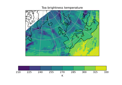
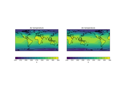
Figure 2 Quickplot of a 2D Cube on a Map

Cross Section Plots

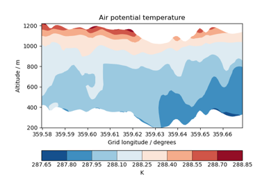
Figure 3 Cross Section Plots

Multi-Line Temperature Profile Plot

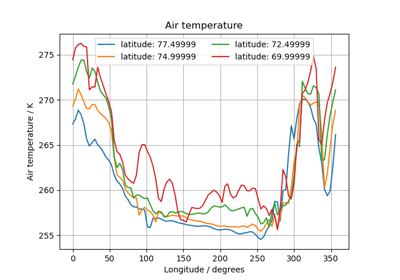
Figure 4 Multi-Line Temperature Profile Plot

Fitting a Polynomial

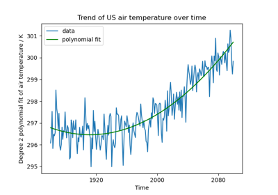
Figure 5 Fitting a Polynomial

Rotated Pole Mapping

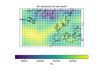
Figure 6 Rotated Pole Mapping

Test Data Showing Inset Plots

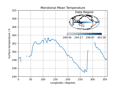
Figure 7 Test Data Showing Inset Plots

Applying a Filter to a Time-Series

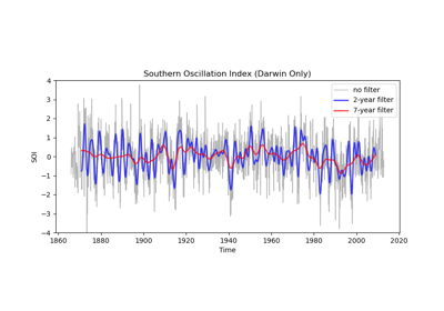
Figure 8 Applying a Filter to a Time-Series

Deriving the Coriolis Frequency Over the Globe

Figure 9 Deriving the Coriolis Frequency Over the Globe

Calculating a Custom Statistic

Figure 10 Calculating a Custom Statistic

Colouring Anomaly Data With Logarithmic Scaling

Figure 11 Colouring Anomaly Data With Logarithmic Scaling

Plotting in Different Projections

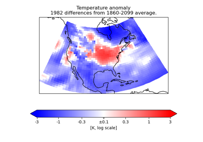
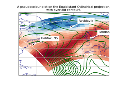
Figure 12 Plotting in Different Projections
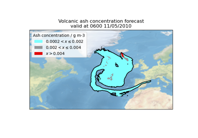
Loading a Cube From a Custom File Format

Figure 13 Loading a Cube From a Custom File Format

Meteorology

Ionosphere Space Weather

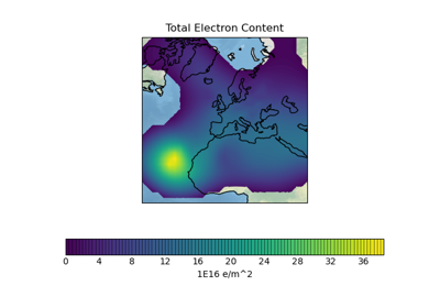
Figure 14 Ionosphere Space Weather

Hovmoller Diagram of Monthly Surface Temperature

Figure 15 Hovmoller Diagram of Monthly Surface Temperature

Plotting Wind Direction Using Quiver

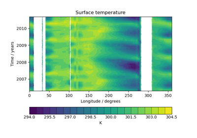
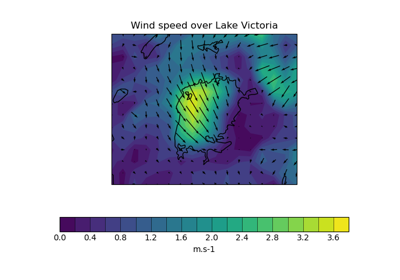
Figure 16 Plotting Wind Direction Using Quiver

Plotting Wind Direction Using Barbs

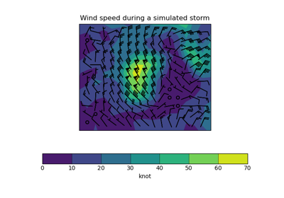
Figure 17 Plotting Wind Direction Using Barbs

Deriving Exner Pressure and Air Temperature

Figure 18 Deriving Exner Pressure and Air Temperature

Global Average Annual Temperature Plot

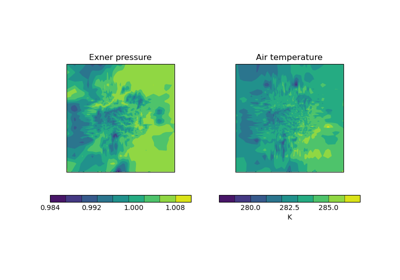
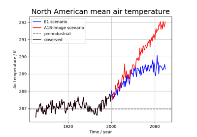
Figure 19 Global Average Annual Temperature Plot

Seasonal Ensemble Model Plots

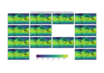
Figure 20 Seasonal Ensemble Model Plots

Global Average Annual Temperature Maps

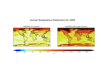
Figure 21 Global Average Annual Temperature Maps

Oceanography

Tri-Polar Grid Projected Plotting

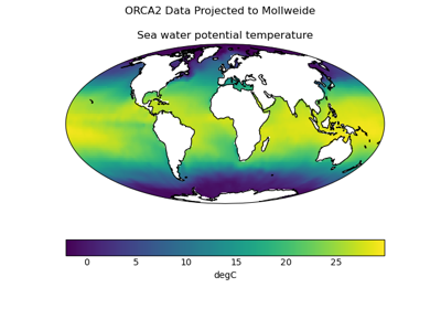
Figure 22 Tri-Polar Grid Projected Plotting

Load a Time Series of Data From the NEMO Model

Figure 23 Load a Time Series of Data From the NEMO Model

Oceanographic Profiles and T-S Diagrams

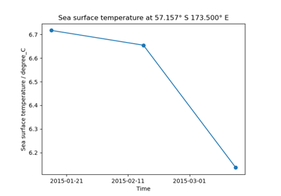
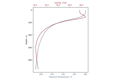
Figure 24 Oceanographic Profiles and T-S Diagrams

Download all examples in Python source code: gallery_python.zip

Download all examples in Jupyter notebooks: gallery_jupyter.zip

Gallery generated by Sphinx-Gallery

previous

Installing

next

Example of a Polar Stereographic Plot

© Copyright 2010 - 2021, Iris Contributors.

Created using Sphinx 4.3.2.

Built using Python 3.8.12.